Experiment →Uncertain situations, which could have multiple outcomes. A coin toss is an experiment.

Outcome → result of a single trial. So, if "head" lands, the outcome of the coin toss experiment is “Heads”

Event → one or more outcomes from an experiment. “Tails” is one of the possible events for this experiment.

Basic Probability

Chance of something happening, but in the academic term “likelihood of an event or sequence of events occurring”. for example

Tossing a coin

Rolling a dice

Conditional Probability

Probability of an event occurring given that another event has already occurred. for example

Picking 3 blue balls from a box has 5 red and 5 blue balls.

The probability of picking the first blue ball is 5/10 = 1/2.

We’re left with 9 balls in total. So the probability of picking the second blue ball is 4/9. Similarly picking the 3rd blue ball from the box is 3/8.

The final probability is 1/2 * 4/9 * 3/8 = 0.08333 or 8.3%.

Probability Density function and Probability Mass Function

The probability distribution for a discrete random variable is the probability mass function (PMF) and the probability distribution for a continuous variable is the probability density function (PDF).In the data science field, countplot is an example of PMF similarly, distplot is an example for PDF.

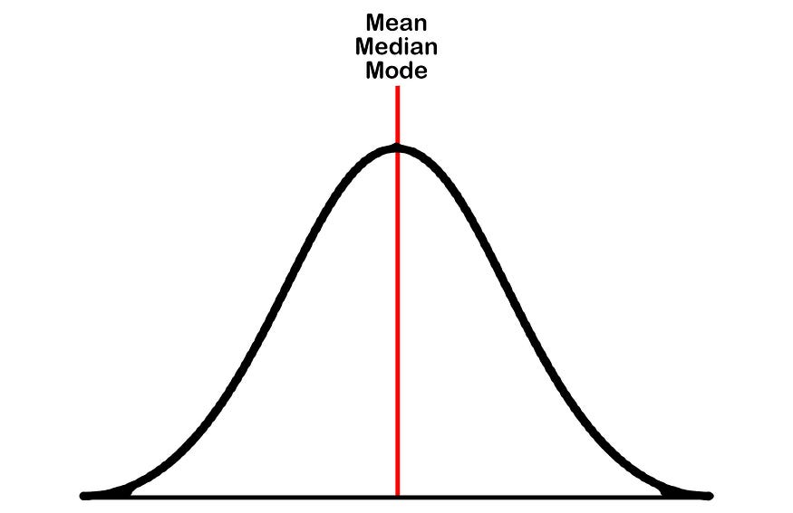
Normal Distribution

Symmetric about the mean

Also known as Gaussian distribution.

Data near the mean are more frequent.

Bell curve-like structure.

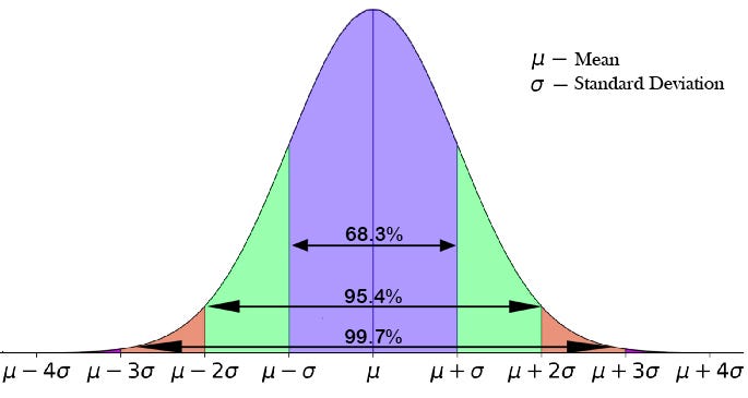
68–98–99.7 Rule

If the data is normally distributed, then we can confidently say that,

68.3 % of the data falls under the 1st standard deviation from the mean.
95.4 % of the data falls under the 2nd standard deviation from the mean.
99.7 % of the data falls under the 3rd standard deviation from the mean.

Z - Score (-3 σ to +3 σ)

The number of standard deviations from the mean, it is also called a standard score or sigma score. Z stands for standard normal distribution.

Population mean and Sample mean

The mean of the entire population dataset is known as the population mean. The mean of sample data which is randomly selected from the population data is known as the sample mean.

Central Limit Theorem (CLT)

Sampling distribution of the mean of any random and independent variable will be normally or nearly normally distributed if the random sample sizes are large enough. Usually, each random sample size should be equal to or greater than 30 will be considered for CLT to hold.

Note: Population can be in any distribution

Confidence Interval (CI)

It is a range of plausible values for an unknown parameter. The interval has an associated confidence level that the true parameter is in the proposed range. It is often expressed a percentage (%) whereby a population means lies between an upper and lower interval.

The 95% confidence interval is a range of values that can be 95% certain contains the true mean of the population. As the sample size increases, the range of interval values will narrow, meaning that the mean with much more accuracy compared with a smaller sample.

Hypothesis Testing

It can be also called AB testing and Confirmative analysis. There are 2 types

Null Hypothesis → general statement or default position that there is no relationship between two measured phenomena or no association among groups

Alternate Hypothesis → Just opposite of the null hypothesis and alternate of the null hypothesis. If the null hypothesis is “I’m gonna win 10000 points” then the alternate hypothesis is “I’m gonna win more than 10000 points”.

Type 1 and Type 2 Error

Type I error is the rejection of a true null hypothesis, while a type II error is the non-rejection of a false null hypothesis. for example,

If the null hypothesis is that the person is innocent, while the alternative is guilty.

In this case, type 1 error is that the person is innocent but sent him to jail
Type 2 error is that the person is guilty but set him free.

Level of significance (α)

Degree of significance in which we accept or reject the null-hypothesis. 100% accuracy is not possible for accepting or rejecting a hypothesis, so we, therefore, select a level of significance that is usually 0.05 or 5%, which means the output should be 95% confident to give a similar kind of results in each sample.

One-tailed test → region of rejection is on only one side of the sampling distribution.

Two tail test → The critical area of a distribution is two-sided and tests whether a sample is greater than or less than a certain range of values. If the sample being tested falls into either of the critical areas, the alternative hypothesis is accepted instead of the null hypothesis.

P-value

Probability of finding the observed, or more extreme, results when the null hypothesis of a study is true. If P-value is less than the chosen significance level (usually 0.05) then we can reject the null hypothesis. P-value is between 0 and 1.

Types of Hypothesis Testing

T-test ( Student T-test)
Z-test
ANOVA Test (F-test)
Chi-Square Test

T-test → We can use when there is a significant difference between the men's of 2 samples which may be related in certain features.

One Sample T-test → We can use to check whether the sample mean is statistically different from the hypothesized population mean or not.
Two Sample T-test → We can use to compare the means of 2 independent samples in order to determine whether there is statistically evident that the associated population means are significantly different or not.
Paired Sample T-test → We can use to check the significant difference between 2 related variables.

Z-test → Same as the T-test but we can use it when the sample size is greater than 30.

Note: We can use T-test in any size of sample data but we can’t use z test if the sample size is lesser than 30.

ANOVA Test (F-Test) → The T-test and Z-test works well when dealing with two groups, but sometimes we want to compare more than two groups at the same time.

One Way ANOVA Test → Tells whether two or more groups are similar or not based on their mean similarity and f-score.
Two Way ANOVA Test → Used when we have 2 independent variables and 2+ groups.

Note: 2-way F-test does not tell which variable is dominant. if we need to check individual significance then Post-hoc testing needs to be performed.

Chi-Squared test (x² test)

It is used to test the relationship between categorical features.

Goodness of fit → Tells whether the distribution of sample categorical feature matches as expected or not. Usually, if the value is greater than 2 then it is a good fit.
Test of Independence → Tells whether two categorical features are independent or not.

Bias

A simplified assumption was made by the model to make the target function easier to learn. On the other hand, bias is the error that we get on training time.

Low bias → less error on the training time.
High bias → high error on the training time.

Variance

An amount that the estimate of the target function will change if different training data was used. In simple terms, variance is the error that we get on testing time.

Low variance → less error on the testing time.
High variance → high error on the testing time.

Note: Low bias and low variance is the goal of any ML model. Linear models often have high bias and low variance. Non linear models often have low bias and high variance.

Underfitted model → Model with high bias and high variance.
Overfitted model → Model with low bias and high variance.

Thank you
Ram Thiagu

Linkedin→ https://www.linkedin.com/in/ram-thiagu/

Search This Blog

Ram Thiagu

Inferential Statistics in Data Science